How To: Analyze and Plot Three Point Shooting Trends

This tutorial goes through the process of generating figures in my Three Point Shooting Trends blog. Please read the blog first before continuing on to the tutorial. In this tutorial you will learn the following:

1. Scrape league average stats for several seasons using nba_api.
2. Plot using plotnine which is a Python port of R's ggplot. This package is how I generate most of my visualizations.
3. Saving data in different formats including: csv, parquet & feather. We'll go through pros and cons of each.
4. Processing data using pandas

If you want to run the code yourself while reading the tutorial, you can find the notebook version of this tutorial on my github:

https://github.com/sravanpannala/NBA-Tutorials/blob/main/three_pt_shooting_trends/plotting_three_pt_shooting_trends.ipynb

First, let's start by loading the basic packages required for this tutorial.

import pandas as pd  # for processing data
import numpy as np  # for numerical operations on arrays
from tqdm import tqdm  # gives up progress bar

# don't raise warnings when chaining pandas operations
pd.options.mode.chained_assignment = None

data_DIR = "./data/"

Plotting Basic 3 PT Year to Year Trends

Scraping the Data

Now, let's load the function required for scraping league average data.

from nba_api.stats.endpoints import leaguedashteamstats

year = 2023
# the function requires season to be in the form "2023-24" instead of "2024"
season = str(year) + "-" + str(year + 1)[-2:]
# Get per game stats for a regular season
stats = leaguedashteamstats.LeagueDashTeamStats(per_mode_detailed="PerGame", season_type_all_star="Regular Season", season = season)
# Get data frames
df = stats.get_data_frames()[0]
# We don't need all columns, so we load only a subset 
df = df[["TEAM_NAME","W","L","W_PCT","FG3M","FG3A","FG3_PCT"]]
df.head(2)

# Sum all the columns and append sum as a new row
df.loc["Total"] = df.sum()
df.tail(1)

# Average the makes and attempts for 30 teams
df.loc["Total","FG3M"] = df.loc["Total","FG3M"]/30
df.loc["Total","FG3A"] = df.loc["Total","FG3A"]/30 
# Get the percentage by dividing makes column with attempts column
df.loc["Total","FG3_PCT"] = df.loc["Total","FG3M"]/df.loc["Total","FG3A"]
# Rename the team_name column entry of total row to the season
df.loc["Total","TEAM_NAME"] = year +1
# round the columns to three decimals
df.iloc[:,4:] = df.iloc[:,4:].round(3)
# get only the last row i.e. the total row
dft = df.tail(1)
dft = dft[["TEAM_NAME","FG3M", "FG3A", "FG3_PCT"]]
dft

Now let's run the above code for the past 10 seasons

dfa = []
for year in tqdm(range(2014,2024)):
    # the function requires season to be in the form "2023-24" instead of "2024"
    season = str(year) + "-" + str(year + 1)[-2:]
    # Get per game stats for a regular season
    stats = leaguedashteamstats.LeagueDashTeamStats(per_mode_detailed="PerGame", season_type_all_star="Regular Season", season = season)
    # Get data frames
    df = stats.get_data_frames()[0]
    # We don't need all columns, so we load only a subset 
    df = df[["TEAM_NAME","W","L","W_PCT","FG3M","FG3A","FG3_PCT"]]
    
    df.loc["Total"] = df.sum()
    df.loc["Total","FG3M"] = df.loc["Total","FG3M"]/30
    df.loc["Total","FG3A"] = df.loc["Total","FG3A"]/30 
    df.loc["Total","FG3_PCT"] = df.loc["Total","FG3M"]/df.loc["Total","FG3A"]
    df.loc["Total","TEAM_NAME"] = year +1
    df.iloc[:,4:] = df.iloc[:,4:].round(3)
    dft = df.tail(1)
    dft = dft[["TEAM_NAME","FG3M", "FG3A", "FG3_PCT"]]
    dfa.append(dft)
df_3pct = pd.concat(dfa)

 80%|████████  | 8/10 [00:06<00:01,  1.14it/s]

100%|██████████| 10/10 [00:08<00:00,  1.17it/s]

# rebane team name column to season
df_3pct = df_3pct.rename(columns={"TEAM_NAME":"Season"}).reset_index(drop=True)
df_3pct

Plotting the Data using Plotnine

Now that we have the data, let's plot it. We'll do it using plotnine package. I recommend reading the documentation and going through the tutorials there.
Let's load the modules from plotnine, we'll use in plotting:

from plotnine import ggplot, aes, geom_line, geom_point, labs

p = (
    # load the dataframe here
    ggplot(df_3pct)
    # define the x and y data i.e. aesthetics
    + aes(x="Season", y= "FG3A")
    # line plot
    + geom_line(group=1)
    # scatter plot
    + geom_point()
    # Set title and caption
    + labs(
            title= "3PT Attempts per Game 2014-2023",
            caption="@SravanNBA | source:nba.com/stats",
        )
)
# draw the plot
p.draw()

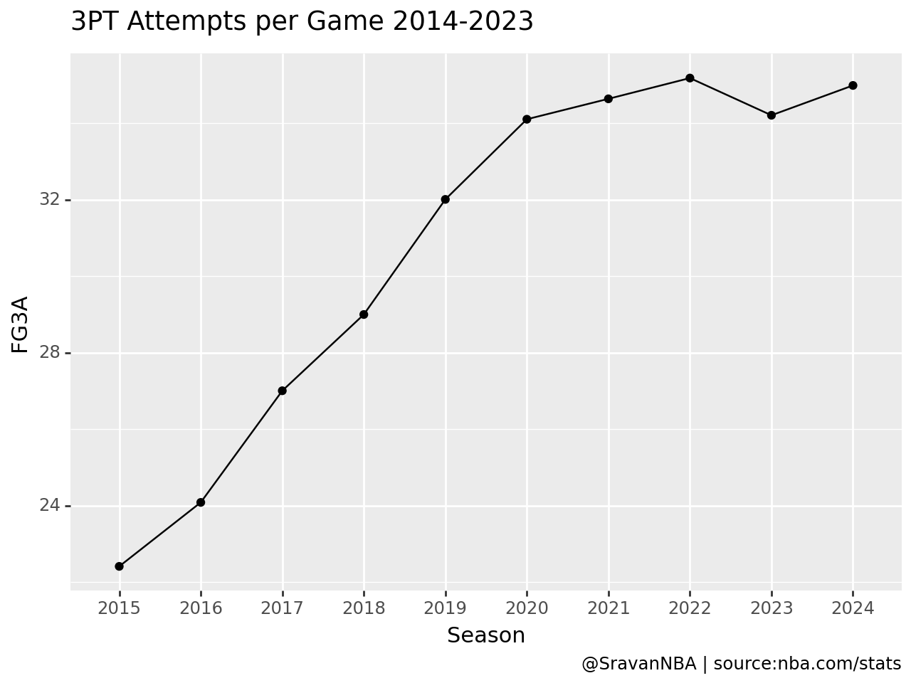
Wow, that was easy. The default plot here is much better formatted compared to a default matplotlib plot. This is what makes using plotnine fun and easy. We need to just worry about the data and then plotnine takes care about the formatting.
Now, lets make the plot even better looking by adding a theme. We need to import some things again from plotnine

from plotnine import themes, theme, element_text

We are going to be using the xkcd theme. For a list of available themes refer to plotnine themes documentation. Let's define the theme now:

theme_idv = themes.theme_xkcd(base_size=11)

I want to slightly modify the theme by making the title bold and increase the title font size to 16. That can be done by updating the theme like so:

theme_idv += theme(
    plot_title=element_text(face="bold", size=16),
)

Now, we add the theme to the previous plot by just adding this line to the code + theme_idv

p = (
    ggplot(df_3pct)
    + aes(x="Season", y= "FG3A")
    + geom_line(group=1)
    + geom_point()
    + labs(
            title= "3PT Attempts per Game 2014-2023",
            caption="@SravanNBA | source:nba.com/stats",
        )
    # adding the new theme
    + theme_idv
)
p.draw()

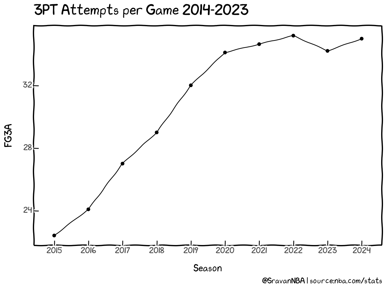
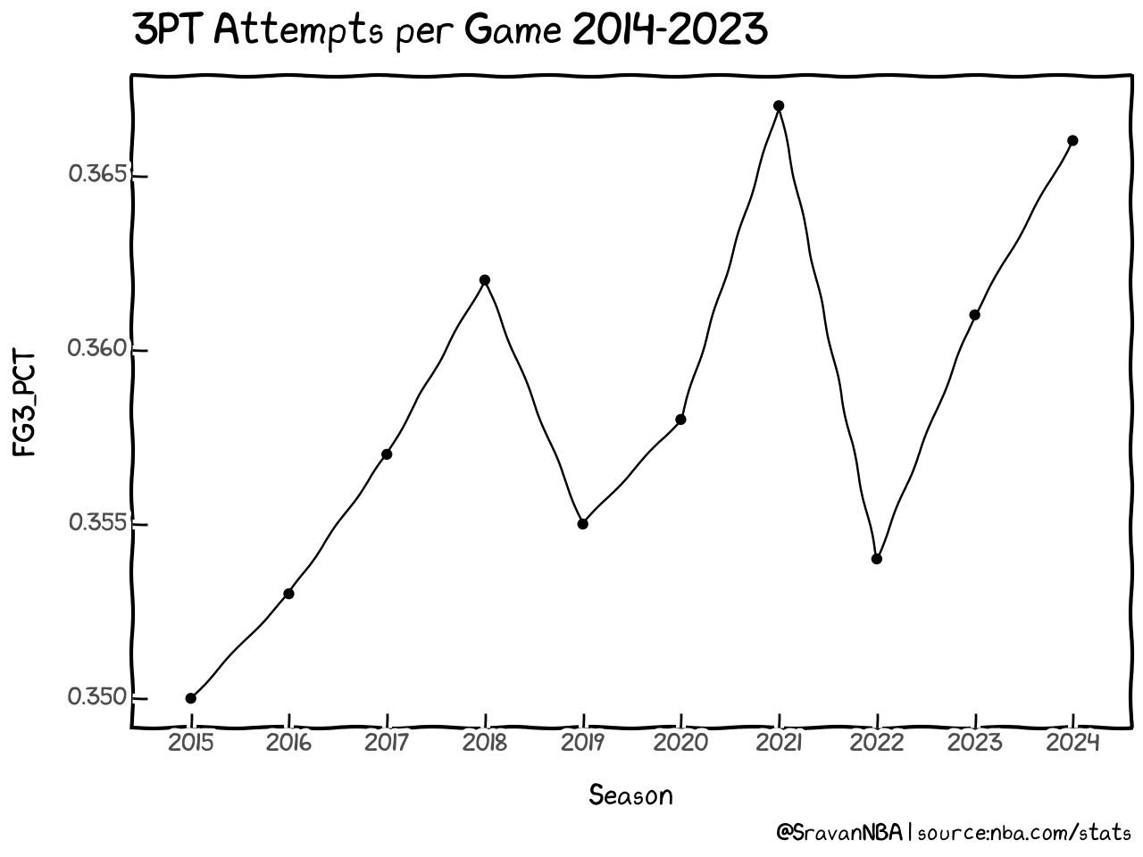
Wasn't that easy? Now the graph with xkcd looks much better than the vanilla theme we saw before. Similarly we can generate plot for 3PT Makes by just changing y="FGM" in the code. For generating 3PT percentage trends, we set y="FG3_PCT". Once you start getting used to plotnine, visualizing data will become much easier.

p = (
    ggplot(df_3pct)
    # we change the y aesthetic here
    + aes(x="Season", y= "FG3_PCT")
    + geom_line(group=1)
    + geom_point()
    + labs(
            title= "3PT Attempts per Game 2014-2023",
            caption="@SravanNBA | source:nba.com/stats",
        )
    + theme_idv
)
p.draw()

3FG% vs Wins Year to Year when Team 3P% > Opponent 3P% + 5%

Scraping Data and saving them in different file formats

Now, let's load the function required for boxscores, which are required to get individual game 3FG% and whether a team has won or not

from nba_api.stats.endpoints import leaguegamelog

season = "2022"
# api call for getting the data
stats = leaguegamelog.LeagueGameLog(
    player_or_team_abbreviation="T",
    season=season,
    season_type_all_star="Regular Season",
)
df = stats.get_data_frames()[0]
# define the file name string
file_name = data_DIR + "NBA_BoxScores_" + "Standard" + "_" + season 

pandas offers us several ways of saving dataframes. The most commonly used one is to_csv() which saves the data in a csv format. csv I want to introduce you to other formats of storing data including parquet and feather.

df.to_csv(file_name + ".csv")
df.to_parquet(file_name + ".parquet")
df.to_feather(file_name + ".feather")

New, let's try to evaluate how long it takes to save the file by using timeit magic function. Read more about jupyter/IPython built-in magic commands here.

%%timeit
df.to_csv(file_name + ".csv")

32.8 ms ± 2.5 ms per loop (mean ± std. dev. of 7 runs, 10 loops each)

%%timeit
df.to_parquet(file_name + ".parquet")

19.3 ms ± 1.31 ms per loop (mean ± std. dev. of 7 runs, 10 loops each)

%%timeit
df.to_feather(file_name + ".feather")

10.3 ms ± 1.83 ms per loop (mean ± std. dev. of 7 runs, 100 loops each)

Time taken to save: feather <parquet < csv
Let's look at the file sizes

import os

file_stats = os.stat(file_name + ".csv")
file_size = file_stats.st_size >> 10
print(f"{file_size} kB")

355 kB

file_stats = os.stat(file_name + ".parquet")
file_size = file_stats.st_size >> 10
print(f"{file_size} kB")

88 kB

file_stats = os.stat(file_name + ".feather")
file_size = file_stats.st_size >> 10
print(f"{file_size} kB")

256 kB

So,File size: parquet < feather < csv

I personally use parquet files over csv for the below reasons:

Parquet Files

• why not csv
  • not compressed, can take too much space
  • doesn't save dtypes, pandas has to infer dtypes after reading the csv. It isn't reliable and sometimes you have to set dtypes manually
• What is parquet

Apache Parquet is an open source, column-oriented data file format designed for efficient data storage and retrieval. It provides efficient data compression and encoding schemes with enhanced performance to handle complex data in bulk.

• why parquet
  • compressed automatically
  • saves dtypes
  • faster to write and load
• disadvantages
  • you can't read the file visually, like you can a csv
  • No proper/popular GUI tool to visualize csv files like Microsoft Excel or Google Sheets

Now let's back to scraping the data:
First we save the data in parquet format for all 10 seasons

season_start = 2014
season_end = 2024
seasons = np.arange(season_start, season_end, 1).astype(str)
for season in tqdm(seasons):
    stats = leaguegamelog.LeagueGameLog(
        player_or_team_abbreviation="T",
        season=season,
        season_type_all_star="Regular Season",
    )
    df = stats.get_data_frames()[0]
    df.to_parquet(data_DIR + "NBA_BoxScores_" + "Standard" + "_" + season + ".parquet")

100%|██████████| 10/10 [00:11<00:00,  1.17s/it]

Processing Data

Let's load data for a season

year = 2023
df = pd.read_parquet(data_DIR + f"NBA_BoxScores_Standard_{year}.parquet")
df.head(2)

Each row, only has that team's data but we need both teams data in a single row to compare 3PT shooting between two teams. To have data for both teams in the same row, we follow same steps as in the previous tutorial.

df = df[["GAME_ID","TEAM_NAME","FG3A","FG3M","FG3_PCT","PLUS_MINUS"]]
df1 = df.groupby("GAME_ID")
df1_1 = df1.nth(0)
df1_2 = df1.nth(1)
df1_1.columns = ["GAME_ID"] + [s + "1" for s in df1_1.columns if s != "GAME_ID"]
df1_2.columns = ["GAME_ID"] + [s + "2" for s in df1_2.columns if s != "GAME_ID"]
df1_3 = pd.merge(df1_1,df1_2)
df1_4 = df1.nth(1)
df1_5 = df1.nth(0)
df1_4.columns = ["GAME_ID"] + [s + "1" for s in df1_4.columns if s != "GAME_ID"]
df1_5.columns = ["GAME_ID"] + [s + "2" for s in df1_5.columns if s != "GAME_ID"]
df1_6 = pd.merge(df1_4,df1_5)
df2 = pd.concat([df1_3,df1_6]).sort_values("GAME_ID").reset_index(drop=True)
df2.head(2)

df3 = df2[["TEAM_NAME1","TEAM_NAME2","FG3_PCT1", "FG3_PCT2","PLUS_MINUS1","PLUS_MINUS2"]]
# 3 Point shooting of team > 5% of opponent
df3["More_3PT_PCT"] = df3["FG3_PCT1"] > (df3["FG3_PCT2"] + 0.05) 
# Define Win and Loss
df3["Win"] = df3["PLUS_MINUS1"] > 0
df3["Loss"] = df3["PLUS_MINUS1"] < 0
# Wins when 3FG% of team > 3FG% of opponent + 5%
df3["Win_More_3PT_PCT"] = df3["More_3PT_PCT"] & df3["Win"]
df3["Loss_More_3PT_PCT"] = df3["More_3PT_PCT"] & df3["Loss"]
# Aggregate all values together for a team
df4 = df3.groupby("TEAM_NAME1")[["Win_More_3PT_PCT","Loss_More_3PT_PCT"]]\
    .agg({"Win_More_3PT_PCT":["sum"],"Loss_More_3PT_PCT":["sum"]})
df4.columns = ["Win_More_3PT_PCT","Loss_More_3PT_PCT"]
df4 = df4.sort_values(by="Win_More_3PT_PCT",ascending=False).reset_index().rename(columns={"TEAM_NAME1":"Team"})
# Sum values from all teams to total row for the season
df4.loc['Total']= df4.sum()
df4.loc['Total','Team'] = "Total"
df4.loc['Total','Team'] = year +1
# get the total row out as a dataframe
dft = df4.tail(1)

Now, we have to run the same process for all 10 seasons

dfa = []
for year in range(2014,2024):
    df = pd.read_parquet(data_DIR + f"NBA_BoxScores_Standard_{year}.parquet")
    df = df[["GAME_ID","TEAM_NAME","FG3A","FG3M","FG3_PCT","PLUS_MINUS"]]
    df1 = df.groupby("GAME_ID")
    df1_1 = df1.nth(0)
    df1_2 = df1.nth(1)
    df1_1.columns = ["GAME_ID"] + [s + "1" for s in df1_1.columns if s != "GAME_ID"]
    df1_2.columns = ["GAME_ID"] + [s + "2" for s in df1_2.columns if s != "GAME_ID"]
    df1_3 = pd.merge(df1_1,df1_2)
    df1_4 = df1.nth(1)
    df1_5 = df1.nth(0)
    df1_4.columns = ["GAME_ID"] + [s + "1" for s in df1_4.columns if s != "GAME_ID"]
    df1_5.columns = ["GAME_ID"] + [s + "2" for s in df1_5.columns if s != "GAME_ID"]
    df1_6 = pd.merge(df1_4,df1_5)
    df2 = pd.concat([df1_3,df1_6]).sort_values("GAME_ID").reset_index(drop=True)
    df3 = df2[["TEAM_NAME1","TEAM_NAME2","FG3_PCT1", "FG3_PCT2","PLUS_MINUS1","PLUS_MINUS2"]]
    df3["More_3PT_PCT"] = df3["FG3_PCT1"] > (df3["FG3_PCT2"] + 0.05) 
    df3["Win"] = df3["PLUS_MINUS1"] > 0
    df3["Loss"] = df3["PLUS_MINUS1"] < 0
    df3["Win_More_3PT_PCT"] = df3["More_3PT_PCT"] & df3["Win"]
    df3["Loss_More_3PT_PCT"] = df3["More_3PT_PCT"] & df3["Loss"]
    df4 = df3.groupby("TEAM_NAME1")[["Win_More_3PT_PCT","Loss_More_3PT_PCT"]]\
        .agg({"Win_More_3PT_PCT":["sum"],"Loss_More_3PT_PCT":["sum"]})
    df4.columns = ["Win_More_3PT_PCT","Loss_More_3PT_PCT"]
    df4 = df4.sort_values(by="Win_More_3PT_PCT",ascending=False).reset_index().rename(columns={"TEAM_NAME1":"Team"})
    df4.loc['Total']= df4.sum()
    df4.loc['Total','Team'] = "Total"
    df4.loc['Total','Team'] = year +1
    dft = df4.tail(1)
    dfa.append(dft)
df_pw = pd.concat(dfa).reset_index(drop=True)
df_pw = df_pw.rename(columns={"Team":"Season"})
df_pw["Win_PCT"] = (df_pw["Win_More_3PT_PCT"]/(df_pw["Win_More_3PT_PCT"]+df_pw["Loss_More_3PT_PCT"])).round(3)

Here is the dataframe which we will plot next

df_pw

p = (
    ggplot(df_pw)
    + aes(x="Season", y= "Win_PCT")
    + geom_line(group=1)
    + geom_point()
    + labs(
            title= "Team Win % When Having 5% higher 3PT% than Opponent",
            caption="@SravanNBA | source:nba.com/stats",
            y = "Win %",
        )
    + theme_idv
    + theme(plot_title=element_text(face="bold", size=15))
)
p.draw()

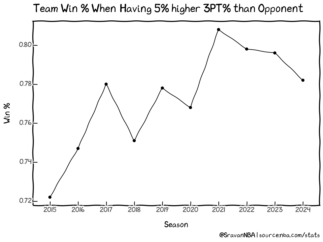
Now, lets format the Y axis to show data in percentage instead of fraction

from mizani.formatters import percent_format
from plotnine import scale_y_continuous

p = (
    ggplot(df_pw)
    + aes(x="Season", y= "Win_PCT")
    + geom_line(group=1)
    + geom_point()
    # Change Y scale to percent
    + scale_y_continuous(labels=percent_format())
    + labs(
            title= "Team Win % When Having 5% higher 3PT% than Opponent",
            caption="@SravanNBA | source:nba.com/stats",
            y = "Win %",
        )
    + theme_idv
    + theme(plot_title=element_text(face="bold", size=15))
)
p.draw()

Finally you can save the figure using the save command

p.save("FG3PCT_Wins_seasons.png", width=6.2, height=4.8, dpi=300)

c:\Users\pansr\AppData\Local\pypoetry\Cache\virtualenvs\nba-ub9Z_EQq-py3.11\Lib\site-packages\plotnine\ggplot.py:587: PlotnineWarning: Saving 6.2 x 4.8 in image.
c:\Users\pansr\AppData\Local\pypoetry\Cache\virtualenvs\nba-ub9Z_EQq-py3.11\Lib\site-packages\plotnine\ggplot.py:588: PlotnineWarning: Filename: FG3PCT_Wins_seasons.png

Reminder

You can find the notebook version of this tutorial on my github: https://github.com/sravanpannala/NBA-Tutorials/blob/main/three_pt_shooting_trends/plotting_three_pt_shooting_trends.ipynb